
Experience Curve Effects: Swanson’s Law, Learning Rate, Component Differences, Cost Drivers, Cumulative Doublings, Formula, Distinction From Scale, Limits, Price Versus Cost, Progress Ratio
Experience curve effects are the pattern in which unit costs fall by a consistent percentage each time cumulative production doubles. Key aspects include learning rate, swanson’s law, cost drivers, component differences, formula, cumulative doublings, limits, distinction from scale, progress ratio, and price versus cost. The usual way to measure this fall is the learning rate, the percentage by which cost drops with each doubling of total output. For solar modules this rate has historically been near 20 percent, and the formula behind it links cost to cumulative volume through a power-law exponent. Swanson’s Law describes the same pattern for photovoltaic modules, noting that prices have dropped roughly 20 percent for every doubling of shipped capacity. Because falling module prices shape project economics, the best solar companies Delaware is a phrase that often appears in discussions of how local installation markets respond to these cost trends. The article goes on to explain the main cost drivers, such as scale, efficiency gains and cheaper materials, and how components like cells, inverters and mounting hardware follow different curves.
Key Takeaways
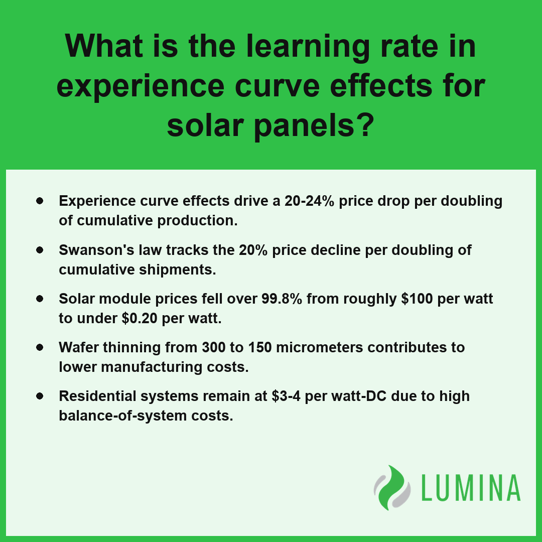
- Experience curve effects drive a 20-24% price drop per doubling of cumulative production.
- Swanson’s law tracks the 20% price decline per doubling of cumulative shipments.
- Solar module prices fell over 99.8% from roughly $100 per watt to under $0.20 per watt.
- Wafer thinning from 300 to 150 micrometers contributes to lower manufacturing costs.
- Residential systems remain at $3-4 per watt-DC due to high balance-of-system costs.
What Is the Learning Rate in Experience Curve Effects for Solar Modules?
The learning rate in experience curve effects for solar modules is the percentage by which the cost of a unit drops with each doubling of cumulative production, which has historically remained at about 20-24 percent. Per the International Renewable Energy Agency, solar photovoltaic module prices have historically demonstrated a learning rate of approximately 20 percent for every doubling of cumulative installed capacity. This metric provides a consistent measure of how process improvements, design changes, and expanded manufacturing output translate into lower prices for you as a purchaser of solar technology. While the learning rate focuses on the efficiency gains during every doubling of cumulative production, it is distinct from simple economies of scale or the labor-focused improvements typically analyzed within a firm’s internal learning curve.
| Metric Category | Learning Rate (Per Doubling) | Industrial Context | Progress Ratio |
|---|---|---|---|
| Solar PV Modules (Historical Range) | 20% – 24% | Renewable Energy Sector | 76% – 80% |
| Standard Industrial Benchmarks | 10% – 30% | General Manufacturing | 70% – 90% |
| Solar PV (IRENA Observed Average) | 20% | Global Installed Capacity | 80% |
Solar Experience Curve: Cost Reductions per Doubling
When you evaluate the impact of the experience curve effect on solar technology, consider how different variables contribute to these historical declines:
- Cumulative Output Growth: Global solar installations have surged from under 1 gigawatt in the early 2000s to well over 2 terawatts, representing roughly eleven or more doublings of capacity.
- Industrial Benchmarks: Across broader industrial sectors, experience curve effects generally yield cost declines of 10-30 percent per doubling, with corresponding progress ratios between 70-90 percent.
- Price Trajectory: Sustained learning rates have driven module prices from roughly $100 per watt in the mid-1970s to well under $0.20 per watt today, amounting to a total decline exceeding 99.8 percent.
Compare the current module price against the total installed cost of your system to determine how much of your investment is currently tied to hardware versus non-module expenses.
Several factors drive the sustained decline in costs beyond simple cumulative production volume:- Supply Chain Optimization: Integration of upstream manufacturing processes reduces material waste and transportation expenses.
- Technological Transitions: Shifts from multi-crystalline to mono-crystalline PERC cells have accelerated efficiency gains that lower cost-per-watt.
- Automation Integration: Increased deployment of high-speed robotic assembly lines minimizes labor overhead and improves precision.
- Material Efficiency: Reductions in silver content and silicon wafer thickness per unit directly lower the commodity cost burden.
- Standardization: Industry-wide alignment on module dimensions and interconnect technologies streamlines installation and balance-of-system costs.
How the Experience Curve Formula C(n) = C1 × n^(-b) Applies to Solar Module Costs
The experience curve formula C(n) = C1 × n^(-b) quantifies the solar module cost reduction you observe as cumulative production increases, showing that every doubling of cumulative production typically drives a cost decline of about 20-24% through the experience curve effect. According to the National Renewable Energy Laboratory, the experience curve formula indicates that for every doubling of cumulative solar photovoltaic production, the cost of modules historically declines by approximately 20 percent.
| Metric | Mathematical Symbol | Definition |
|---|---|---|
| Cost of nth unit | C(n) | Unit cost after reaching specific cumulative production volume |
| Initial Unit Cost | C1 | Baseline cost of the first manufactured unit |
| Cumulative Production | n | Total count of units produced since inception |
| Experience Exponent | b | Numerical factor dictating the slope of cost reduction |
| Progress Ratio | 2^(-b) | Percentage of original cost retained after doubling output |
| Learning Rate | 1 – 2^(-b) | Percentage of cost reduction achieved per production doubling |
Solar Cost Reduction Metrics
What Do the Terms in the Formula Mean?
The formula C(n) = C1 × n^(-b) represents the experience curve effects by mapping unit costs to historical growth. In this mathematical model, C(n) signifies the cost of the nth unit produced, while C1 represents the cost of the very first unit. The variable n stands for the cumulative production of solar modules, and b is the experience exponent that dictates the speed of cost reduction. By calculating these variables, you can determine how reliably an industry converts cumulative manufacturing experience into lower prices.
How Do Progress Ratio and Learning Rate Connect to the Exponent?
The connection between your progress ratio and learning rate is anchored in the exponent b, which governs the steepness of the cost decline curve. You can evaluate the efficiency of production improvements through these two specific indicators:
- Progress Ratio: 2^(-b), representing the fraction of cost remaining after a doubling of cumulative production.
- Learning Rate: 1 − 2^(-b), representing the percentage cost reduction achieved with each doubling of cumulative production.
Reading the Exponent From a Typical Solar Module Decline
For a solar module, the typical industrial experience curve often reflects a learning rate near 20-24 percent. If you observe a progress ratio of 80 percent, you are effectively seeing an exponent b of approximately 0.32, which results in a 20 percent cost drop per doubling.
Which Doubling of Cumulative Production Figures Fit Solar?
Solar module history fits the model well, as global installations have surged from under 1 gigawatt to well over 2 terawatts. This growth trajectory confirms the following patterns regarding the doubling of cumulative production:
- Total expansion: Roughly eleven or more doublings have occurred.
- Price evolution: Module costs dropped from roughly $100 per watt in the mid-1970s to well under $0.20 per watt.
- Consistent decline: The observed 20-24% drop per doubling persists across these eleven cycles.
Compare the historical cost-to-volume exponent of your specific solar technology against industry-standard benchmarks to identify if your current procurement prices are tracking with expected experience curve effects.
The following drivers contribute to the cost reductions observed in the experience curve:- Economies of scale: Spreading fixed costs over a larger volume of units produced.
- Process innovation: Adopting more efficient manufacturing techniques and automated assembly methods.
- Supply chain optimization: Negotiating better bulk pricing for raw silicon and secondary components.
- Product redesign: Simplifying module architecture to reduce material intensity and labor time.
- Increased labor efficiency: Improving workforce productivity through repetitive tasks and specialized training.
Swanson’s Law and Its Link to Experience Curve Effects in Solar
Swanson’s law is a specific manifestation of experience curve effects within the solar industry, positing that the price of a solar module drops by about 20% for every doubling of cumulative production. According to BloombergNEF, this law effectively tracks how the price of photovoltaic modules tends to decline by approximately 20 percent for each doubling of cumulative shipped capacity. While the broader experience curve effect applies to a wide range of industrial sectors with cost declines between 10% and 30%, Swanson’s law serves as a consistent empirical observation of how historical price trends follow the predictable patterns of mass manufacturing and scaling. By observing that global module prices fell from roughly $100 per watt in the mid-1970s to well under $0.20 per watt, a decline of more than 99.8%, you can see the profound impact of cumulative volume on market economics.
| Metric Category | Learning Rate (Price Reduction per Doubling) | Contextual Application |
|---|---|---|
| Industry Upper Limit | 30% | Broad industrial experience curve peak |
| Swanson’s Law | 20% | Solar photovoltaic module specific trend |
| Industry Lower Limit | 10% | Broad industrial experience curve baseline |
Solar Price Decline per Doubling of Capacity
- Experience curve effect: A broad economic principle applied to any industry where costs decline as experience accumulates.
- Swanson’s law: A solar-specific rule documenting that module prices fall by approximately 20% with each doubling of cumulative shipments.
- Scope of impact: Swanson’s law focuses on the price of the module itself, whereas the experience curve effect tracks the cost trajectory of all value-added components.
This relationship highlights why rapid growth in global capacity, which has seen cumulative installations rise from under 1 gigawatt in the early 2000s to well over 2 terawatts, has effectively driven prices downward across eleven or more doublings. To gauge the potential for future price volatility, analyze how recent module price trends align with the historical 20-24% decline rate observed during previous cycles of market growth.
Several key factors contribute to the sustained cost reductions observed in the solar industry beyond simple cumulative volume:- Technological improvements in silicon purification and wafer-thinning techniques that reduce material waste.
- Efficiencies of scale in manufacturing facilities, leading to lower overhead costs per unit.
- Increased automation in panel assembly processes, reducing labor costs and human error.
- Global supply chain optimizations that drive down the logistics and procurement expenses for raw materials.
- Standardization of cell architectures, such as the shift from PERC to TOPCon, which accelerates production speed and output quality.
Technology and Manufacturing Changes Behind Solar Experience Curve Effects, From Thinner Wafers to Diamond-Wire Cutting
Technology and manufacturing changes drive experience curve effects by systematically removing material waste and optimizing conversion processes at each doubling of cumulative production. You can track these advancements through the evolution of silicon usage and precision engineering, which have collectively pushed module efficiency from about 12% to over 21-23%. According to the Department of Energy, advances in automated manufacturing processes and high-throughput production lines have enabled greater economies of scale and efficiency gains in the assembly of solar modules within the domestic market. These technical refinements minimize the raw materials required per watt, ensuring that every factory expansion yields a greater output relative to the input costs.
| Manufacturing Optimization Metric | Historical Standard | Modern Technical Standard | Efficiency Impact |
|---|---|---|---|
| Silicon Wafer Thickness | 300 μm | 150 μm | Reduced raw material consumption per watt |
| Cutting Technology | Slurry-based sawing | Diamond-wire cutting | Minimized kerf loss and increased slicing speed |
| Metallization Usage | High silver paste density | Optimized thin-line printing | Lower material cost per unit of power |
| Production Capacity | Megawatt-scale purification | Multi-gigawatt capacity | Realized economies of scale in manufacturing |
Silicon Wafer Thickness Evolution (μm)
- Wafer dimensions: Larger silicon wafers allow for more efficient handling and cell processing during manufacturing.
- Wafer thickness: Precision sawing has reduced thickness from about 300 micrometers to about 150 micrometers, significantly lowering silicon consumption per cell.
- Diamond-wire cutting: This technology has replaced older slurry-based methods, enabling faster slicing with thinner kerf losses and reduced material waste.
- Cell chemistry: Continuous innovation in cell design has optimized light absorption, requiring less silver paste per cell to achieve higher power output.
- Factory scale: Moving from megawatt-scale to multi-gigawatt capacity in polysilicon purification plants has enabled massive gains in operational efficiency.
Examine the technical specifications of a module datasheet to determine if the manufacturer utilizes thin-wafer or diamond-wire cutting technologies to sustain their competitive cost structure.
Recent advancements in solar module fabrication reflect a broader shift toward maximizing material efficiency through several strategic technical upgrades:- Implementation of bifacial module architectures to capture reflected light from the rear surface without increasing cell footprint.
- Transition to large-format wafer sizes, such as M10 and M12, to reduce the relative cost of frame and glass materials per watt.
- Integration of Passivated Emitter and Rear Cell (PERC) technology to improve internal quantum efficiency and light trapping.
- Adoption of multi-busbar designs to decrease electrical resistance and reduce the silver contact area required for current collection.
Why Module Prices Fall Faster Than the Installed Cost of Residential Systems
Module prices fall faster than the installed cost of residential systems because the experience curve effects that drive massive cost reductions in high-volume, global manufacturing do not apply uniformly to the localized, labor-intensive components of a home-based setup. While the solar module is a global commodity benefiting from gigawatt-scale production, residential installations rely heavily on balance-of-system costs and soft costs that remain stubbornly resistant to automation and standardization. Per Lawrence Berkeley National Laboratory, non-hardware soft costs now account for the majority of total residential system prices in the United States, establishing a cost floor that prevents module-level price drops from fully lowering consumer-facing quotes.
| Cost Category | Primary Driver of Price | Sensitivity to Experience Curves | Scalability Potential |
|---|---|---|---|
| Solar Hardware | Global commodity manufacturing | High (Gigawatt-scale reductions) | Exponential |
| On-Site Labor | Localized site-specific assembly | Low (Physical/Manual constraints) | Stagnant |
| Soft Costs | Regulatory, design, and permitting | None (Institutional complexity) | Often Increasing |
The discrepancy between declining hardware prices and stable installation costs is best understood by looking at the components that define a residential project:
- Hardware: Includes the solar module and inverter, both of which benefit significantly from experience curve effects and economies of scale.
- Labor: Includes mounting, electrical wiring, and physical assembly, which involve site-specific challenges that prevent meaningful long-term cost declines.
- Soft Costs: Include local permitting, inspection, design, and financing requirements, which often increase in complexity or remain stagnant regardless of manufacturing improvements.
When you evaluate a quote for a new system, distinguish between the module cost, which tracks with global progress ratios, and the balance-of-system costs, which often dominate your final invoice and do not share the same historical trajectory of decline.
Assess how much of your total investment is tied to hardware efficiency gains versus fixed local labor and administrative charges.
Several distinct factors contribute to the persistence of high soft costs in residential solar projects:- Permitting Variations: Disparate local building codes and inspection requirements prevent the adoption of a universal, streamlined design standard.
- Customer Acquisition Expenses: High marketing, lead generation, and sales commission costs reflect the fragmented nature of the retail consumer market.
- Interconnection Procedures: Inconsistent utility policies regarding grid integration force bespoke engineering solutions for individual residential properties.
- Financing Complexity: High underwriting and administrative overhead associated with residential solar loans and lease agreements add significant premiums to the total contract price.
Frequently Asked Questions
What does a progress ratio of 0.8 mean for solar panel experience curve effects?
A progress ratio of 0.8 means that for every doubling of cumulative production, your costs decline by 20%. This metric represents the cost remaining after a doubling, falling within the typical industrial progress ratios of 70-90% that characterize the experience curve effect in various manufacturing sectors.
How many cumulative doublings has solar PV capacity gone through, and what does that mean for the experience curve?
Solar PV capacity has gone through roughly eleven or more doublings as global installations grew from under 1 gigawatt in the early 2000s to well over 2 terawatts. This volume accounts for the dramatic price decline of more than 99.8% observed since the mid-1970s.
Will the solar panel experience curve keep going or hit a floor from material costs and efficiency limits?
The experience curve effect is descriptive rather than guaranteed, meaning it does not automatically continue; cost reductions depend on ongoing innovation. While advancements like thinner silicon wafers, now at about 150 micrometers, and higher cell efficiencies have driven past gains, future progress faces physical limits and shifting input prices.
Do solar panel price drops during oversupply make experience curve effects look steeper than real cost learning?
Yes, solar panel price drops during oversupply can make experience curve effects appear steeper because market price versus cost fluctuations often decouple. While long-term trends follow learning, short-term market dynamics, policy-driven demand, and supply gluts can temporarily accelerate price declines beyond the underlying progress in manufacturing efficiency.
Is the experience curve effect the same as economies of scale or the learning curve in solar panel manufacturing?
No, the experience curve effect is not the same as economies of scale or the learning curve. The learning curve focuses on labor hours per unit, and economies of scale relate to output rates at a point in time, while the experience curve covers all value-added costs across cumulative production.